


What OpenCLIP Did to My Photo Library
27th May 2026 • 12 min read — by Aleksandar Trpkovski
Play audio summary
I love taking photos. I've been at it for years now - landscapes, cityscapes, astrophotography, coastal scenes, mountains, seascapes, waterfalls. The kind of photography where you set an alarm for 3am to catch the Milky Way, where you wait for the right tide at the right beach, and where you drive for a few hours out of town just because the light might be good.
Naturally, my photo library kept growing. Faster than I could keep up with.
When I decided to publish those images to my website, I realised I needed a better way to organise them. I came up with a gallery organised into six themed buckets:
- Starlit Wonders
- Wild Horizons
- Time in Motion
- Urban Glow
- Ocean Whispers
- Liquid Cascades
I could categorise these shots by hand. Not a big deal with 110 photos. But I thought, let's see if I can use some modern tools to do it for me - not just for the photos I have now, but for every new shot I'll add to the library in the future.
The obvious modern answer is "throw it at an AI." But I didn't want to pay per call to a frontier model so I went looking for an open-source alternative.
What I found was much more interesting than what I went looking for. By the end of the weekend I'd given one open-source model my entire library and built four small things on top of it.
Let me show you what happened.
Meet OpenCLIP
OpenAI released a model called CLIP back in 2021. The easiest way to understand why it's different from a normal image classifier is by what it isn't.
A normal image classifier is taught a fixed list of things at training time. Say you trained it on cats, dogs, and rabbits - those three categories are now its entire world. Show it a hamster and it'll confidently call it a rabbit, because that's the closest option it has. It can't shrug. It doesn't even know that it doesn't know.
CLIP doesn't live behind those walls. You can describe almost anything to it in plain English - "a photo of a hamster", "a foggy mountain at dawn", "a starry sky over the ocean" - and it'll know what to look for, even though nobody sat down and specifically taught it those categories. No list to update, no retraining to run. You describe what you want, and it goes looking.
OpenAI published the paper and the weights, but kept the training code and dataset private.
OpenCLIP is the open-source community response, built by LAION and ML Foundations. Same architecture, but trained on bigger, fully open datasets, with open code you can actually reproduce and fine-tune. The current best OpenCLIP checkpoints comfortably outperform OpenAI's original weights on almost every benchmark. The one I picked for this project, ViT-H-14 / dfn5b, hits around 83% zero-shot ImageNet accuracy and produces a 1024-dimensional vector for every image it sees.
You don't need to understand all of that to use it. You need to know two things: it's free, and it's surprisingly good.
Teaching It My Categories Without Training Anything
The first thing I wanted was to sort my library into those six themed buckets. The traditional way to do this would be to label hundreds of my own photos per category and train a classifier. I wasn't doing that.
CLIP has a better trick called zero-shot classification. Instead of training on labelled data, you describe your categories in plain English at the moment of asking. The model looks at every image and picks the description that best matches.
The model has never heard of "Starlit Wonders" - that's my poetic name. But it has seen plenty of starry-sky photos with descriptive captions during its training, so the moment I give it a concrete prompt like "a photo of the night sky full of stars", it knows what to match against.
In practice this meant defining each category as a list of plain-English prompts rather than a single label:
"Starlit Wonders": [
    "a photo of the night sky full of stars",
    "astrophotography of the milky way",
    "a starry night sky over a landscape",
    "a long exposure photo of star trails",
]
"Wild Horizons": [
    "a landscape photo of wild nature",
    "a scenic view of mountains and forests",
    "an untouched wilderness landscape",
    "a wide nature vista with green hills",
    "a national park scenery photo",
    ],
"Time in Motion": [
    "a long exposure photograph showing motion blur",
    "light trails from moving traffic at night",
    "a photo with motion blur showing the passage of time",
    "a time-lapse style long exposure photograph",
    "blurred movement captured in a single photograph",
],
"Urban Glow": [
    "a city skyline glowing at night",
    "an urban street with neon lights at night",
    "city lights and skyscrapers after dark",
    "a nighttime cityscape photo",
    "a glowing urban scene at dusk",
],
"Ocean Whispers": [
    "a calm ocean seascape",
    "waves on the sea coastline",
    "a photo of the open ocean",
    "a tranquil beach and sea view",
    "the surface of the ocean at golden hour",
],
"Liquid Cascades": [
    "a photo of a waterfall",
    "water cascading down rocks",
    "a flowing river with rapids",
    "a tall waterfall in a forest",
    "cascading water in nature",
    ],
The model averages the embeddings of all the prompts in the list before comparing against each photo - a technique called prompt ensembling.
Under the hood, the script does the same thing for every photo: load the model once, turn each image into a 1024-dim vector, turn the category prompts into vectors in the same space, then take the similarity between each pair. The category with the highest similarity wins:
import open_clip, torch
from PIL import Image

model, _, preprocess = open_clip.create_model_and_transforms(
    "ViT-H-14", pretrained="dfn5b"
)
tokenizer = open_clip.get_tokenizer("ViT-H-14")
model.eval()

image = preprocess(Image.open("photo")).unsqueeze(0)
prompts = tokenizer(["a photo of a waterfall", "a city skyline at night"])

with torch.no_grad():
    img_vec = model.encode_image(image)
    txt_vecs = model.encode_text(prompts)
    similarities = (img_vec @ txt_vecs.T).squeeze()
The first run downloads the model weights (~3.8 GB) into ~/.cache/huggingface/, every subsequent run is instant. That same model.encode_image() call is what powers every other part of the project too.
I ran the whole thing across 110 photos in about thirty seconds.
Classified as Starlit Wonders with confidence 1.0. The model could not have been more decisive.
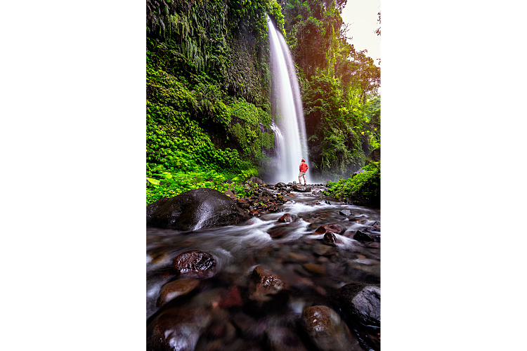
Classified as Liquid Cascades with confidence 0.9998. A classic forest waterfall - exactly what the model was trained to recognise.
It wasn't flawless. A few photos genuinely confused the model:
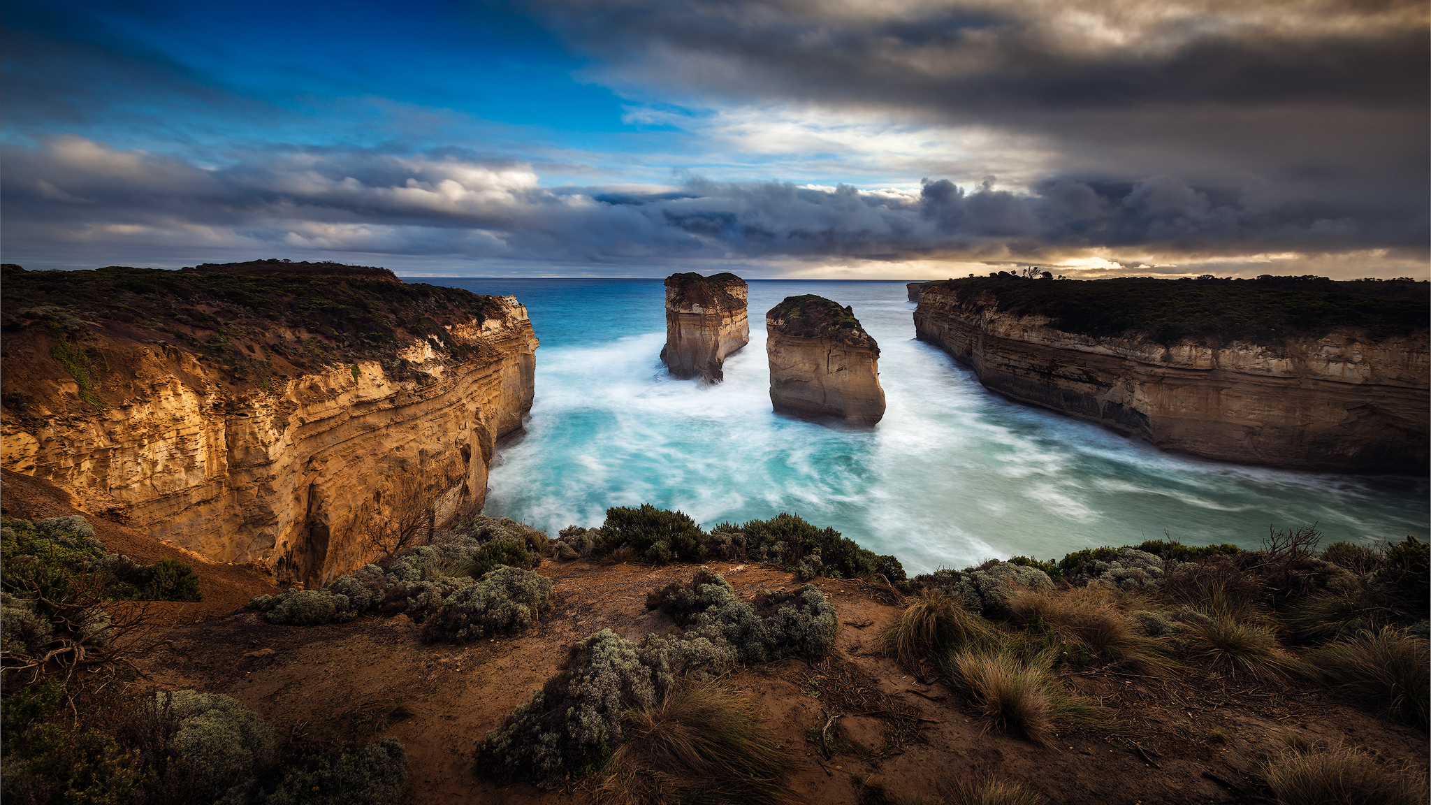
The famous Lord Arch on the Great Ocean Road got classified as Liquid Cascades instead of Ocean Whispers. It's a sea arch, not a waterfall - but the curved rock walls and the rushing water below apparently read more like "cascade" than "coastline" to the model. The confidence margin was thin (0.45 vs 0.33 for the runner-up), so the model wasn't certain either - which is exactly what the margin column in the output CSV is for. Anything with a small margin is worth a manual look.
There was also one case that landed on the right category, but only just:
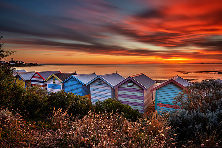
Classified as Ocean Whispers with confidence 0.43. The model got it right - it really is a beach - but the margin over the runner-up was only 0.13. Three categories (Ocean Whispers, Time in Motion, Urban Glow) all took a meaningful slice of the probability budget. The colourful bathing boxes against water genuinely look like multiple things at once.
What the output actually looks like
Each photo gets a row in a CSV with the full breakdown. Here are four rows from my run that together show what the columns mean:
| Milky Way at Pinnacles | Erskine Falls | Lord Arch | Brighton Beach | |
|---|---|---|---|---|
| Predicted category | Starlit Wonders | Liquid Cascades | Liquid Cascades (wrong) | Ocean Whispers |
| Confidence | 1.0000 | 0.9998 | 0.4520 | 0.4318 |
| Margin | 1.0000 | 0.9996 | 0.1240 | 0.1297 |
| Uncertain | False | False | False | False |
| Starlit Wonders | 1.0000 | 0.0000 | 0.0049 | 0.0398 |
| Wild Horizons | 0.0000 | 0.0002 | 0.1711 | 0.0179 |
| Time in Motion | 0.0000 | 0.0000 | 0.0440 | 0.3020 |
| Urban Glow | 0.0000 | 0.0000 | 0.0000 | 0.2083 |
| Ocean Whispers | 0.0000 | 0.0000 | 0.3280 | 0.4318 |
| Liquid Cascades | 0.0000 | 0.9998 | 0.4520 | 0.0001 |
What each row of the table means:
- Predicted category is whichever of the six prompts scored highest for that image.
- Confidence is the probability of the winning category, on a 0-1 scale. A confidence of 1.0 means the model thinks there's no reasonable alternative, 0.45 means it's barely above the field.
- Margin is the gap between the top score and the runner-up. This is the real signal of whether the model is sure. A margin of 1.0 means a decisive win, a margin of 0.12 means it almost went the other way.
- Uncertain is a boolean flag that flips to True when the margin drops below a threshold (I used 0.05). Handy for filtering "review by hand" rows.
- The six category columns show each category's softmax score for that image. They sum to 1.0 across each row, so they're really sharing one probability budget. When all six are tiny except one, the model is confident. When the top two are close together, the model is essentially flipping a coin between them.
The Milky Way row tells the whole story in five zeros and one 1.0 - the model had no doubt. Compare it to the Lord Arch row, where four of the six categories have non-trivial scores: the model genuinely couldn't decide. Brighton Beach is the most interesting case: the model picked the right category (Ocean Whispers, since it really is a beach photo), but only just - Time in Motion and Urban Glow were both within striking distance. Low confidence and low margin don't always mean wrong, sometimes they just mean unsure.
Photos as Points in Space
After the experiment with the auto-tagging, the thing I really wanted was to search my library.
This is where embeddings come in, and the easiest way to understand them is with a small analogy. Imagine every photo plotted as a single point in space. Photos of waterfalls cluster together. Astrophotography clusters together. City lights cluster together. The distance between any two points tells you how meaningfully similar the photos are. I explain a bit more in details in the following blog article of me Create a Recommendation Engine with AI for Free, refer to that to learn more about embeddings and how to use them as a recommendation engine.
OpenCLIP turns every image into one of these points. In our case it's a list of 1024 numbers - a single position in a 1024-dimensional space. You can't visualise it, but the maths still works the same way it would in two dimensions. The distance between two points in that space is a measure of how similar the photos are. If you type a sentence like "foggy mountain at dawn" and turn it into a point in the same space, the photos closest to that point are the ones that best match the description.
To make this practical I needed somewhere to store all those vectors and search them quickly. That's exactly what pgvector is for. It's a Postgres extension that adds a vector column type and a few special operators for "find the rows closest to this vector". I ran it in Docker:
cd embeddings && docker compose up -d
The schema is one table with a vector(1024) column. Then a small Python script walks every photo in my images/ folder, encodes it with the same OpenCLIP model, normalises the resulting vector, and inserts it into the database. About a minute for the whole library.
Searching is then literally one line of SQL:
SELECT filename FROM image_embeddings ORDER BY embedding <#> $1 LIMIT 12;
The <#> is pgvector's inner-product operator. Smaller value = closer to the query. The $1 is whatever vector I want to search for - the embedding of a typed sentence, or the embedding of an uploaded photo.
That's the whole retrieval engine in one line. If you want to know more about pgvector refer to the official GitHub repo.
A Little Search App
Once I had embeddings in a database, building a UI around them was the fun bit. I wanted two interactions:
- Type a phrase like "foggy mountain at dawn" and get matching photos back.
- Drop any image into the browser and get visually similar photos back.
Both work the same way under the hood: encode the input with OpenCLIP, run the SQL query above, return the matches.
The architecture is deliberately boring. FastAPI on the backend loads the model once at startup and exposes two endpoints (one for text search, one for image upload). Vite + vanilla TypeScript + Tailwind CSS on the frontend - no React, no framework, just plain DOM. The Vite dev server proxies API calls to FastAPI.
One thing worth mentioning: I originally wanted the whole app in TypeScript. I quickly learned that OpenCLIP doesn't have a clean JavaScript runtime - the Xenova ports of CLIP exist but they're OpenAI's older weights, not the open-source ones I was using, and the vector spaces wouldn't match. The pragmatic answer is to let Python own the model end-to-end and keep the frontend a thin client.
A typed query returns the most semantically similar photos in around 200 milliseconds.
What surprised me is how naturally it understands intent. Typing "loneliness at the edge of the world" surfaced my most isolated coastal shots. Typing "streaks of light across a dark city" pulled up the long-exposure light-trail shots from Melbourne. The model isn't doing any keyword matching - those words don't appear anywhere in my data. It's just measuring distances in meaning space.
Dropping an image is even more striking. Take a photo of any waterfall from the internet, drag it onto the page, and within half a second I'm looking at every waterfall in my own library. Same for cityscapes, beaches, star trails.
One small refinement worth mentioning: I added a similarity threshold so the app only returns results that genuinely match. Without it, every search returns the same number of results regardless of how good the matches actually are - the top three might be relevant, the bottom nine might be noise. With a cosine-similarity floor of about 0.20 for text queries (and a stricter 0.45 for image-to-image, because image embeddings sit closer together in CLIP space), only photos that meaningfully match show up. If nothing crosses the threshold, the app falls back to showing the single closest match so the user always sees something - with a status message that says "no strong matches found."
The full source for the backend and the frontend is in the GitHub repo under search-app/.
Seeing the Library as a Cluster Cloud
Search was the practical win. But there was still something I wanted to see: when CLIP places each photo as a point in 1024-dimensional space, what does that space actually look like? Do my waterfalls really cluster together? Are city lights really far from starry skies? I wanted to look at the geometry directly.
Which immediately runs into a problem.
The 1024-into-3 problem
We see the world in three dimensions. Each photo lives at a point in 1024 dimensions. To draw the cloud on a screen, I need to compress 1024 numbers down to 3 per photo - the x, y, and z coordinates of the dot.
That's a huge compression. We're throwing away 99.7% of the original information. Something has to give.
The cleanest analogy is a globe and a flat map. Earth is a 3D sphere, a paper map is 2D. The moment you flatten the sphere, something has to give - usually the relative size of things. On most world maps you've seen, Russia and Greenland appear far larger than they actually are - Greenland looks roughly the same size as Africa, when Africa is in fact about 14 times bigger. There's no clever way around it, flattening a globe always distorts something. Going from 1024D to 3D is exactly the same situation, just dramatically more extreme.
You can't avoid the loss. You can only choose what you're willing to give up.
Three ways to flatten a thousand dimensions
There are three mainstream algorithms for this kind of dimensionality reduction. Each one makes a different bargain.
PCA (Principal Component Analysis) finds the three directions in 1024D space along which the data spreads out most, and projects everything onto them. It's deterministic, fast, and mathematically interpretable. Its weakness is that it's linear - if your data sits on a curved manifold (which image embeddings absolutely do), PCA flattens that curve awkwardly and the result tends to look like a featureless blob. The top three components often capture only 20-40% of the total variance for high-dim embeddings, so more than half of the structure becomes invisible.
t-SNE does something cleverer. Instead of preserving global geometry, it tries to preserve neighbourhoods: if photo A is one of photo B's nearest neighbours in 1024D, the algorithm tries hard to keep them as nearest neighbours in 3D too. It does this by gradient descent, nudging the 3D positions until the neighbourhood structure matches. The clusters t-SNE produces look tight and well-separated, which is great. But there are big catches: the distances between clusters are meaningless, the result is stochastic (different random seeds give totally different layouts), and there's no way to project a new point onto an existing layout without re-running the entire algorithm.
UMAP (Uniform Manifold Approximation and Projection) combines what's good about both. It preserves local neighbourhoods like t-SNE, but also retains a meaningful chunk of the global structure - meaning the relative positions of clusters to each other carry information, not just within-cluster relationships. It works by first building a graph of each point's nearest neighbours in the high-dim space, then finding a 3D layout that produces a similar graph. It's fast (well under a second on a hundred photos), it has a real transform() method for projecting new points without recomputing everything, and with a fixed random seed it's reproducible.
I picked UMAP. It was the only one that gave me both visible clusters and meaningful inter-cluster geometry on this kind of data. PCA gave me a blob. t-SNE gave me isolated cluster islands floating in a meaningless void. UMAP gave me a cluster cloud where both "what's in a cluster" and "how clusters relate" carried information.
The interactive viewer
Once the projection was working, the visualisation itself came together quickly. A small Python script reads every embedding from pgvector and runs UMAP. The actual call is short:
import umap

reducer = umap.UMAP(
    n_components=3,
    n_neighbors=15,
    min_dist=0.1,
    metric="cosine",
    random_state=42,
)
coords_3d = reducer.fit_transform(embeddings_1024)  # shape: (110, 3)
metric="cosine" matches how the embeddings were normalised. random_state=42 keeps the layout reproducible across runs, which matters because UMAP is non-deterministic by default. The output is written to a JSON file that a Vite frontend (same vanilla TypeScript + Tailwind pattern as the search app) loads and renders with Three.js - one dot per photo, coloured by its predicted category from the classifier earlier.
You can drag to orbit the camera, scroll to zoom, and click any dot to open the underlying image with its metadata in a side panel. Hovering shows the filename in a tooltip. Six colours - one per category - make the cluster reading instant.
Each dot is a photo. Same colour = same predicted category. The spatial grouping is purely a consequence of the underlying CLIP embeddings - the colour is just a confirmation that what the model "sees" matches what we'd expect.
The first time I rotated the camera around it, the experience was genuinely satisfying. There was an obvious cluster of teal dots in one corner - all my waterfalls. A separate purple cluster - astrophotography. The two were on opposite sides of the cloud, which is exactly how my visual instinct would have arranged them. Photos that span multiple categories (long-exposure waterfalls, for example) sit on the boundaries between clusters, slightly pulled by both. That's the model showing me its internal logic, visually.
A few clusters that surprised me
Some neighbour-pairings the visualisation revealed were obvious - waterfall next to waterfall, star trail next to star trail. Others were quietly delightful.
These two sit close together in the cluster cloud even though they were shot in different states, on different trips, years apart. The model picked up on the small wooden boat house, the wooden walkway leading out across the water, and the calm reflective surface beneath - and decided they belonged together visually. I would never have grouped them by hand.
Three waterfall shots from completely different parts of the world, all sitting in the same tight knot of the cluster. The model has never seen a globe. It just recognises "long-exposure cascading water surrounded by green".
One important caveat lives in the corner of the UI: 3D positions are a UMAP approximation - clusters are honest, exact distances are not. When you need precise similarity between two specific photos, the search app is the source of truth. The visualisation is for impression, not measurement.
What This Unlocks
The thing I came away with isn't really "look at this cool app". It's a quieter realisation: this kind of capability has become genuinely commodity.
A model that can match arbitrary natural-language descriptions to arbitrary images now downloads in a few minutes, runs on a laptop, and lets a hobby photographer build a personal search engine over their own library on a Saturday afternoon. There's no API key. There's no monthly bill. Nothing leaves my machine.
The same vectors I generated for search could power "more like this" recommendations on the gallery, detect near-duplicate uploads, or even cluster the library to discover natural groupings I didn't define. That's the architectural payoff of choosing CLIP-style embeddings over a one-shot AI call - you get a representation you can reuse for many features, not just an answer to a single question.
Open-source vision models are quietly some of the most useful tools out there, and they don't get nearly the attention proprietary models do.
The complete code is on my GitHub.
Further Reading
Explore more articles that might interest you.